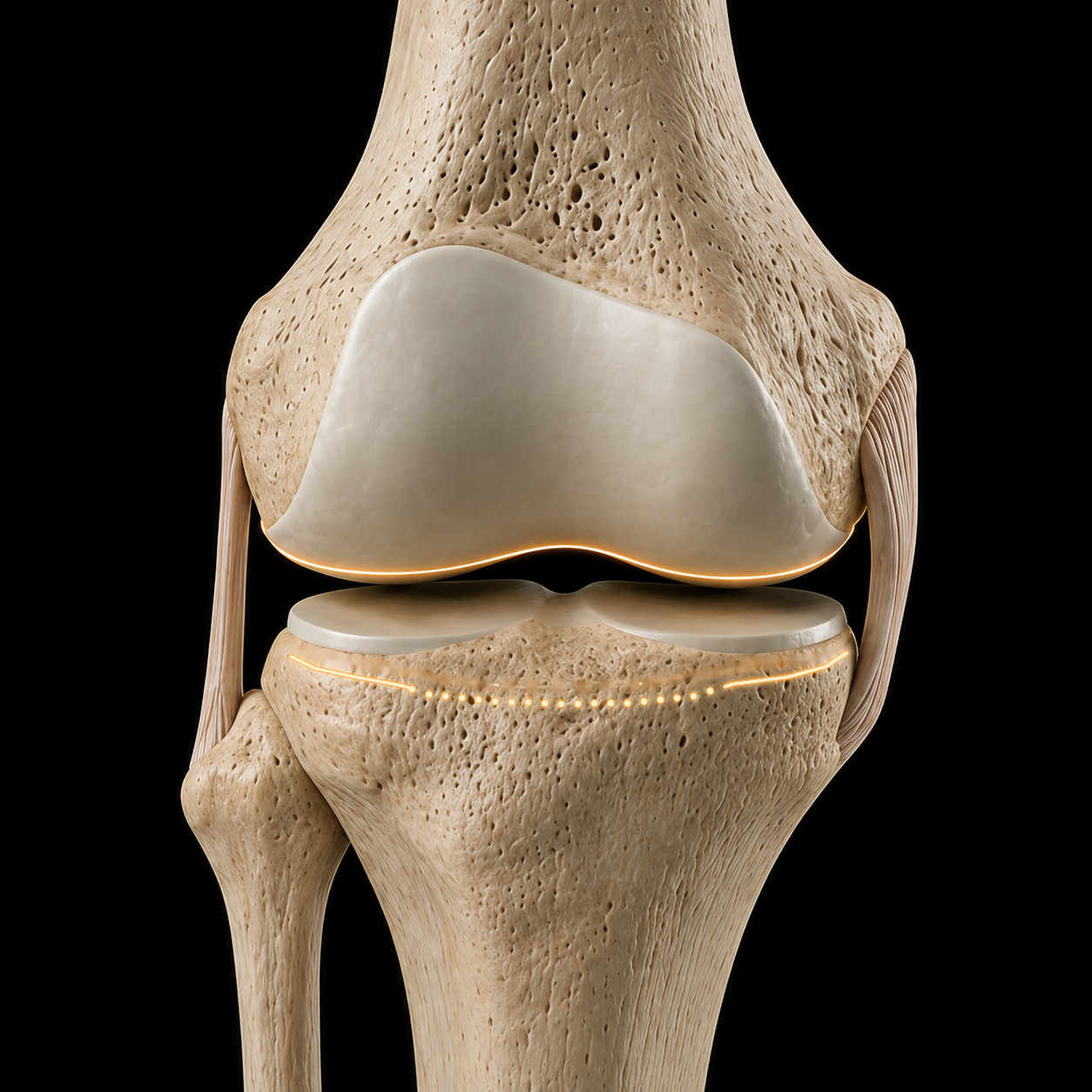
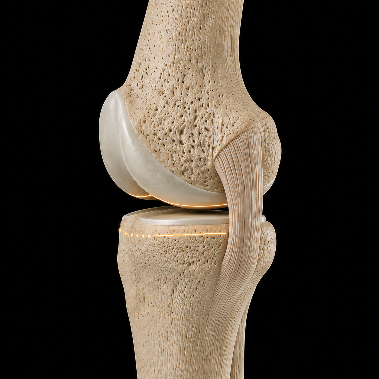
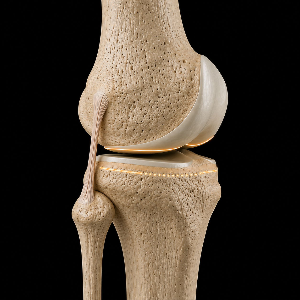
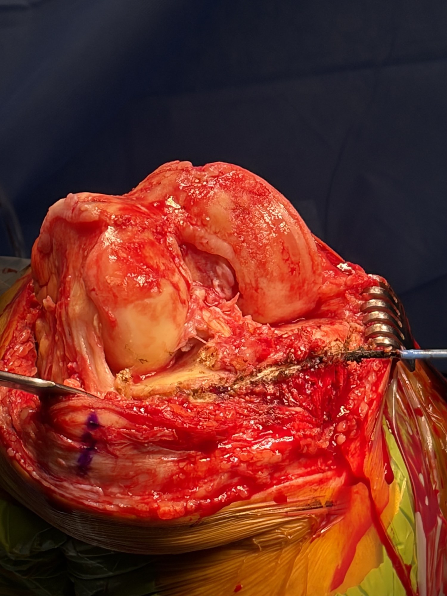
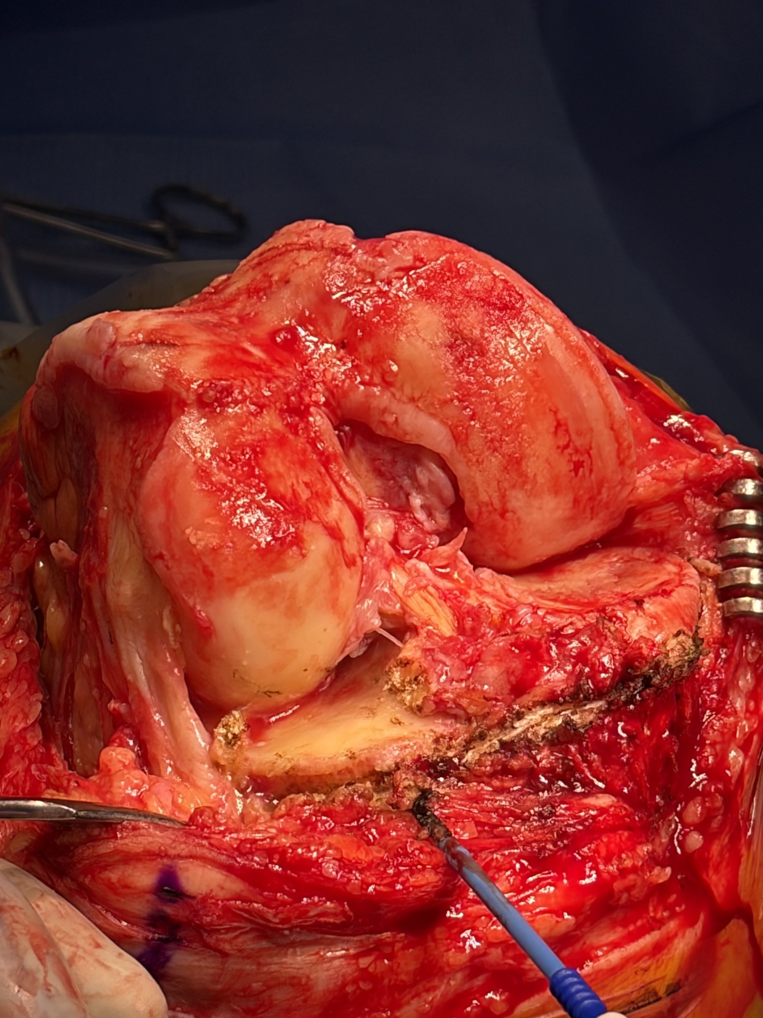
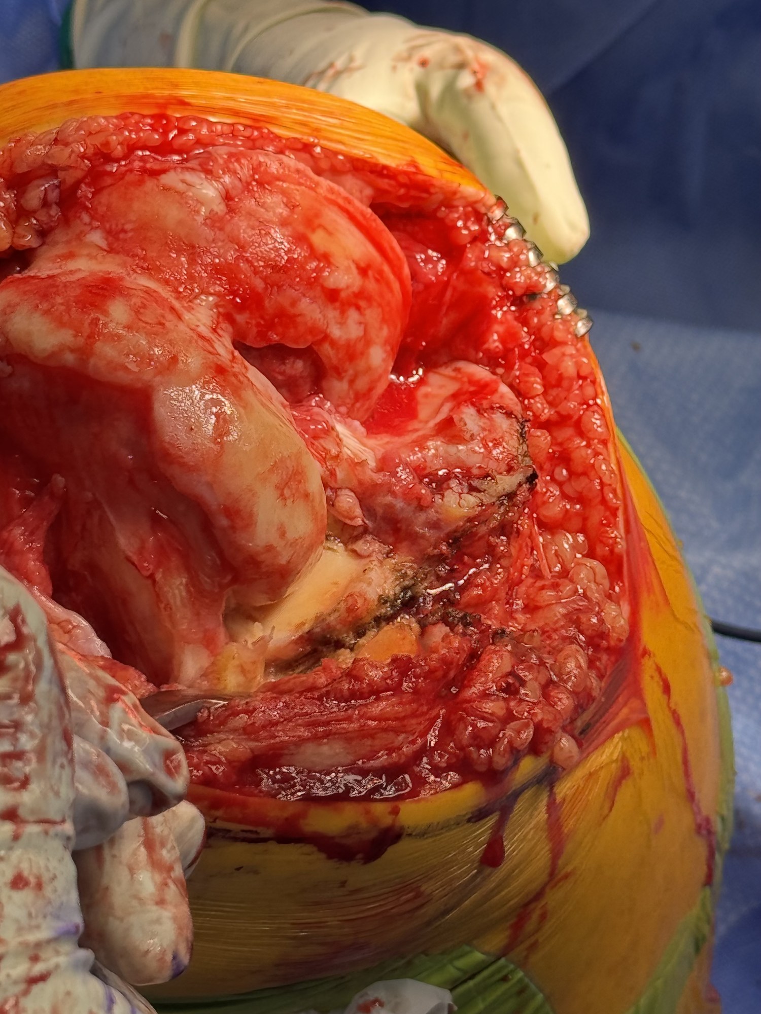
Restore the femoral surface. Restore the tibial surface. Anatomical landmarks guide reconstruction of the articular surface positions present before arthritis.
Trochlear cartilage · Anatomic Tibial LineDrag to change view
Anatomic resurfacing, step by step.
Explore both surfaces, understand the wear, and reconstruct the femoral and tibial surfaces.
The anatomy is the reference.
01 · Anatomic Knee Resurfacing
Restore the femoral surface. Restore the tibial surface.
Anatomical landmarks guide reconstruction of the articular surface positions present before arthritis. Each bone provides its own reference.
Femoral referenceTibial referenceAnatomical view
Loading knee anatomy…
Cartilage-covered surfaces
Each bone has an original articular surface.
Follow the continuous cartilage over the femoral condyles and the cartilage on the tibial plateaus.
Original shells remain attached to their respective bones. Use “Expose surfaces” for a separated inspection view. This illustration does not measure contact pressure or predict knee motion.
Model and reference limits
Open Knee(s), specimen oks009. This reuses the continuous anterior cartilage surface and retained posterior bearing anatomy from the established cartilage illustration. The coating and wear are educational geometry, not a measured thickness map. Preparation and component placement are simplified. Menisci and ACL are omitted; restoration of surface position does not establish native mechanics. The tibial markers reference the model’s medial cartilage surface at one selected location; they do not prescribe a cut or validate a landmark. The insert is a simplified bearing, not manufacturer CAD. Geometry sources and license.
Femoral landmarks
Read the bone. Account for the cartilage.
Distal and posterior femoral landmarks help locate the original articular surfaces. Reconstruction must account for the cartilage that remains and the cartilage and bone that have been lost.
Tibial landmarks
Find the attachments. Recover the reference.
The deep MCL and lateral capsular attachments provide anatomical references for the tibial reconstruction. Joint-line height and coronal orientation are considered together; native slope requires a separate sagittal assessment.
Find both surface references. Reconstruct their positions. Verify how they function together.
01Find
Use femoral bone landmarks and tibial soft-tissue landmarks to estimate the native articular relationship.
02Resurface
Match the reconstruction to that reference, accounting for wear, resection, saw kerf and implant thickness.
03Verify
Measure the reconstruction and assess ligament balance, stability and motion with the trial components.
Howell’s foundation: three axes and the native joint lines
Stephen Howell, Joshua Roth and Maury Hull described kinematic alignment through the relationship between the natural joint lines and three kinematic axes: tibiofemoral flexion–extension, patellofemoral flexion–extension, and tibial internal–external rotation.
Their work explicitly describes resurfacing to restore the natural joint lines. Active Knee Resurfacing places the operative emphasis on finding those references on both the femur and tibia and reconstructing the articular surfaces back to them.
Anatomical rationale supports the reconstruction goal. Restoring the joint line alone does not establish normal kinematics or superior clinical outcomes.
Explore the landmark-to-surface reconstruction example
Bone + soft tissue → joint line
AP · condyle close-up
Loading the enlarged knee…
Distal medial · 0.5 mmOther femoral cartilage · 2 mm
Begin with the femoral condyles and cartilage intact. The gold line marks the joint-line reference.
Cartilage is modeled at 0.5 mm distal medial, 1.5 mm posterior medial, and 2 mm elsewhere on the femur, with smooth transitions between regions. These are illustrative thicknesses. The 9 mm dimensions illustrate this reconstruction, not measurements of the source knee or a universal surgical target. The exposed femoral plane and soft-tissue attachment markers are illustrative. Confirm anatomy, implant thickness and resections in the surgical field. Existing model: Open Knee(s), oks009 ↗
The target
Resurface to the patient’s joint line.
Traditional mechanical alignment targets a neutral reconstruction. Anatomic Resurfacing targets the joint line that belonged to this knee before arthritis.
Follow one example: a native 5° varus joint line, a level mechanical-alignment reconstruction, then a resurfaced knee returned to its original angle and height.
The dotted gold line is the native reference. The solid line follows the reconstructed joint surface.
This retrospective comparison evaluated radiographic restoration. The between-group difference in joint-line obliquity change was not statistically significant (p=0.09); clinical benefit was not established.
Arthritis has worn the surfaces. The dotted gold line marks this knee’s pre-arthritic 5° varus orientation—not a target for every knee.
Illustrative AP comparison, not surgical planning. JLO means joint-line obliquity relative to the horizontal reference shown, not overall leg alignment. Elevation is shown for this example; mechanical alignment does not necessarily raise the entire joint line. The 5° target is specific to this illustration.
The cylindrical axis
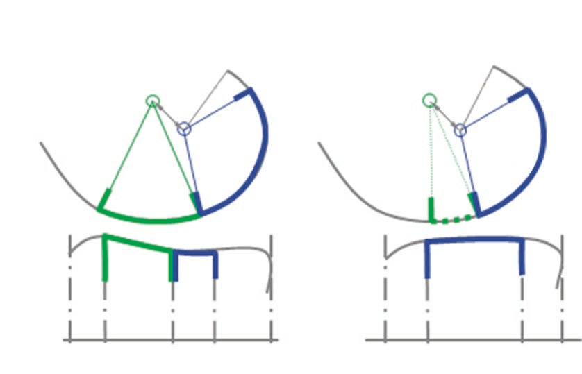
The axis behind the joint line.
Restore the surface–axis relationship. Height. Orientation. Condylar contours.
01 / 03
Two surfaces. One approximate axis.
Two translucent cylinders reveal different condylar radii sharing the blue axis. The orange arcs remain as surface references.
4.6°Mean difference between axes in 3D 23 cadaveric knees · range 1.8°–11.3°
Eckhoff et al. demonstrated that the epicondylar reference and cylindrical axis are distinct. Restoring the tibial joint-line angle alone does not establish restoration of the femoral axis.
Illustrative surface and axis overlays on an anatomical model; these are not measurements or a patient-specific cylinder fit. The medial and lateral radii may differ while sharing an axis. Orange arcs are idealized posterior condylar surface references, distinct from the tibial joint line. Blue spokes show their radii. Eckhoff’s cylinders were fitted to CT-derived bone surfaces corresponding to approximately 15–115° of flexion, not a measured cartilage envelope. These overlays are not a prescribed cut.
The cylindrical axis is an anatomical approximation of the flexion–extension axis. The animation uses the existing anatomical model and illustrative flexion pattern. The axis, contour and spokes move with the femur; they are not a measured kinematic axis, a validated implant design, or a prediction of clinical outcomes. The model does not establish that restoring this geometry alone improves clinical outcomes.
Eckhoff 2005 and 2007 report matching sample sizes and axis-difference statistics; they are not presented here as independent confirmations. Hollister’s and Freeman’s complete axis models differ and are not combined into one validated model.
Existing anatomical model · illustrative motion and axis references
Cartilage
Cartilage · the missing millimetres
Account for wear. Restore the surface.
Cartilage loss changes the reference for femoral resurfacing. Distinguish remaining cartilage, estimated wear and bone loss when planning the original surface level.
Original joint line Planned surface level
Outer sideInner side
Planning lines over native anatomy. Offsets enlarged for clarity.
A teaching example
Cartilage lost 3 mmAccounted for 2.0 mm
1.0mm
Too high.
Underestimating the missing cartilage places the planned femoral surface above its original level.
1 mm2 mm3 mm · target4 mm
Where the correction is applied
A thickness error shifts the surface level.
The joint line helps determine how the surfaces and ligaments work together. Restoring it means accounting for the tissue that is missing.
Illustrative anatomy and planning arithmetic. The 3 mm example is not a measurement of this knee or a standard correction for every patient. Bone loss and other surgical factors also matter.
Cartilage thickness · evidence and planning limits +
Imaging · 25 knees
An X-ray shows the space.
Cartilage is seen directly on MRI. X-ray joint space is an indirect measurement influenced by cartilage, the menisci and positioning. Loading changes the measurements, but does not make them interchangeable.
Femoral cartilage wear followed recognizable patterns in straight and bent positions. Femoral bone wear was uncommon in this study. This does not mean every arthritic knee has no bone loss, particularly on the tibia.
Unworn femoral cartilage averaged 2.0–2.2 mm, with variation between patients and locations. Remaining cartilage provides clues to the original surface; it cannot establish the exact thickness of every worn area.
These studies help explain the anatomical goal of restoration. They do not show that cartilage measurement alone guarantees better function. Assessment also considers bone loss, alignment and the soft tissues.
Planning context: assess distal and posterior femoral wear separately. The demonstration isolates a cartilage estimate; it does not calculate bone resection, implant thickness or saw kerf, and does not model ligament balance.
Ligaments guide the knee throughout movement. Different fibers lengthen and shorten as it bends. Restoring the native joint line aims to preserve the relationship between the joint surfaces and the ligaments.
Normal laxity varies with flexion, loading and the individual. Check the relationship throughout the bend.
Preparing the moving knee…
One ligament. Different fibers.
Each fiber follows its own path.
Anterior MCL fibersLengthen with flexion
Posterior MCL fibersShorten with flexion
Observed during walking, downhill walking and stair descent in healthy knees.
Colored paths illustrate the pattern. They are not measured strain or tension.
Illustrative anatomy and motion. No force scale, surgical target or prediction of an individual result.
Normal is asymmetric.
Healthy knees can open more laterally than medially in flexion under stress.
Normal is individual.
One person’s laxity does not define the target for another.
Geometry matters.
Joint-line height, inclination and bearing thickness are distinct changes.
What the animation shows
The normal view illustrates the direction of anterior and posterior MCL length changes reported during functional activities. These paths are not digitized study data. The LCL is on the opposite side of the knee and is not shown; its behavior varied between subjects.
The comparison is a simplified, exaggerated medial-view model: the elevated reconstruction changes the distal femoral envelope and effective hinge and adds bearing thickness. It illustrates mid-flexion slack with balanced endpoints, not the isolated effect of changing an insert. Identical native and restored motion represents the restoration goal, not a guaranteed postoperative result. Joint-line inclination is not simulated. Read the cadaver study ↗
10 healthy subjects; fluoroscopy-driven models. Anterior MCL fibers lengthened and posterior fibers shortened with flexion. Lengths were normalized to heel strike; absolute strain and ligament forces were not measured.
20 healthy knees near 90° flexion: mean lateral opening 6.7 mm under varus stress, medial opening 2.1 mm under valgus stress. Stress was not standardized and the compartments were stressed separately; these values are not TKA gap targets.
8 non-arthritic cadaveric knees. Medial contact loads exceeded lateral loads and decreased with flexion in the thigh-pull setup. Compartment contact force is not isolated collateral-ligament force or a walking load.
10 cadaveric knees, 0–120° flexion. Passive motion limits varied between knees; most comparisons between directions were not strongly correlated. Results depend on the applied loads and passive test conditions.
267 healthy knees tested with 10 Nm varus and valgus torque at 0° and 15°. Laxity varied between people and increased with flexion. This young, healthy cohort does not establish universal postoperative targets.
A cadaveric TKA reconstruction study found increased mid-flexion laxity after joint-line elevation despite maintained endpoint balance. This supports the illustrated mechanism, not a universal height-to-tension rule.
8 matched cadaver pairs. Kinematic alignment reproduced native mid-flexion MCL strain more closely than mechanical alignment in this experiment. It compared reconstruction strategies and did not isolate inclination alone or measure patient outcomes.
Remove the planned femoral and tibial bone, then replace those surfaces with the femoral component and tibial implant. Account for cartilage wear, bone resection and saw kerf when matching implant thickness.
Watch the gold joint line and ligament attachment points stay fixed as the bone comes out and the implants go in. The goal is to restore the native joint line and ligament relationship—not move them to fit the implant. Confirm the final soft-tissue balance during trialing.
Gold line: native joint-line reference at 3° varus in this example. Gold points: unchanged collateral ligament attachments. The thicker tibial resection is matched by a thicker tibial implant, seated deeper without raising the joint line. The anterior and distal femoral pieces separate before the femoral component is seated. Resections are grouped for clarity, not shown in operative order. This is an illustrative example, not a prescribed angle or resection depth. The goal is to restore the native relationship; ligament tension must still be checked.
Illustrative animation · not a patient-specific model or a measurement of ligament force. Anatomy and operative decisions require clinical verification.
Anatomic landmarks
Femoral anatomy · cartilage & bone
See the wear. Find the bone.
Compare the distal and posterior surfaces. Account for cartilage at each reference.
Cartilage thickness enlarged 3× for visibility. Bone size is unchanged. Thin cartilage is translucent. Both views use the same femur.
Distal surfaceExtension reference
Preparing the femoral surfaces…
Medial0.05 mm
Lateral1.8 mm
Medial wear. Lateral cartilage remains.
Lateral 1.8 mm
Medial 0.05 mm
Posterior surfaceFlexion reference
Preparing the femoral surfaces…
Medial1.5 mm
Lateral1.9 mm
Posterior medial cartilage often remains.
Medial 1.5 mm
Lateral 1.9 mm
Remaining cartilageBone
Illustrative cartilage on the existing femur, not a patient measurement. Numbers are mean remaining cartilage before removal; the small profiles compare those means on one scale. Distal and posterior bone are revealed together.
Remaining cartilage · study values and limits
Nam et al., 2014 · 154 varus and 54 valgus knees with advanced (KL 3–4) osteoarthritis. Values are mean remaining femoral cartilage, in millimetres.
Reference
Varus medial
Varus lateral
Valgus medial
Valgus lateral
Distal · 0°
0.05 mm
1.8 mm
1.5 mm
0.2 mm
Posterior · 90°
1.5 mm
1.9 mm
1.9 mm
0.8 mm
Distal and posterior wear must be assessed separately. The appearance and thickness vary between knees. These data do not specify tibial cartilage thickness, ligament tension, or the clinical effect of a 1 mm difference.
Johnson/Ford (2025) also found variable preservation: the posterior medial femur was judged unworn in 45% of varus knees; the posterior lateral femur was unworn in 33% of valgus knees. “Worn” does not mean absent.
The lateral capsule above Gerdy’s tubercle and the deep MCL insertion at the mid-coronal plane of the tibia serve as references for varus/valgus orientation and tibial cut depth.
MedialDeep MCL insertion
LateralCapsule above Gerdy’s tubercle
Anatomic Tibial Line
Medial
Deep MCL insertion at the mid-coronal plane.
Lateral
Capsular attachment above Gerdy’s tubercle.
Anatomic Tibial Line
Connect the references to guide orientation and depth.
Conceptual educational render. Confirm landmarks directly in the surgical field.
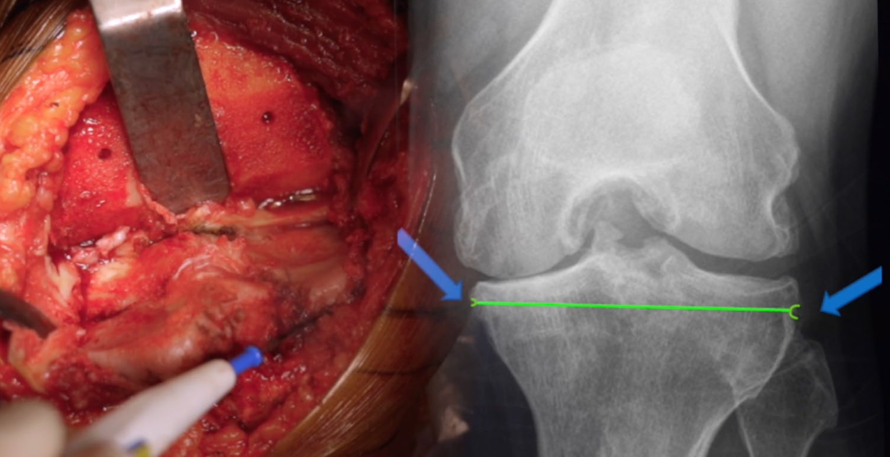
The Tibial Signature · Radiographic reference
Radiographic signature.
From the surgical field to the AP radiograph.
Archives of Orthopaedic and Trauma Surgery · Knee Arthroplasty
Specific tibial landmarks to improve to accuracy of the tibial cut during total knee arthroplasty. A case control study
Sébastien Parratte, Zakee Azmi, Jeremy Daxelet, Jean-Noël Argenson, Cécile Batailler.
These studies do not establish that Active Knee Resurfacing as a complete technique delivers faster recovery or better outcomes than other knee replacements.
Compare the distal and posterior surfaces. Account for cartilage at each reference.
Cartilage thickness enlarged 3× for visibility. Bone size is unchanged. Thin cartilage is translucent. Both views use the same femur.
Distal surfaceExtension reference
Preparing the femoral surfaces…
Medial0.05 mm
Lateral1.8 mm
Medial wear. Lateral cartilage remains.
Lateral 1.8 mm
Medial 0.05 mm
Posterior surfaceFlexion reference
Preparing the femoral surfaces…
Medial1.5 mm
Lateral1.9 mm
Posterior medial cartilage often remains.
Medial 1.5 mm
Lateral 1.9 mm
Remaining cartilageBone
Illustrative cartilage on the existing femur, not a patient measurement. Numbers are mean remaining cartilage before removal; the small profiles compare those means on one scale. Distal and posterior bone are revealed together.
Remaining cartilage · study values and limits
Nam et al., 2014 · 154 varus and 54 valgus knees with advanced (KL 3–4) osteoarthritis. Values are mean remaining femoral cartilage, in millimetres.
Reference
Varus medial
Varus lateral
Valgus medial
Valgus lateral
Distal · 0°
0.05 mm
1.8 mm
1.5 mm
0.2 mm
Posterior · 90°
1.5 mm
1.9 mm
1.9 mm
0.8 mm
Distal and posterior wear must be assessed separately. The appearance and thickness vary between knees. These data do not specify tibial cartilage thickness, ligament tension, or the clinical effect of a 1 mm difference.
Johnson/Ford (2025) also found variable preservation: the posterior medial femur was judged unworn in 45% of varus knees; the posterior lateral femur was unworn in 33% of valgus knees. “Worn” does not mean absent.
The 6 mm resections illustrate this technique, not a universal target. Account for implant thickness, cartilage wear and saw kerf; verify with calipers.
Find the attachments. Connect the line. Match the slope.
01 / 04Medial attachment · proximal tibia
Medial attachment · proximal tibiaIllustrative · not to scale
Illustrated attachment locations require confirmation in the surgical field. The anterior dotted segment connects the reference sites; it is not a strip of capsule.
AP exposureView full size ↗AP exposure · second viewView full size ↗Lateral exposureView full size ↗Tibial cut23 seconds
Verify the reconstruction
Trialing. Evaluating the extension balance.
With the knee in extension, assess medial and lateral stability between the femoral component and tibial polyethylene. Reassess the cuts, component position and soft tissues when the balance is not right.
This view compares extension balance. Then assess mid-flexion and flexion—the same gap pattern is not required at every angle.
Both components remain seated on bone, with no exaggerated opening between the bearing surfaces.
Illustrative animation · not a patient-specific model or a measurement of ligament force. Anatomy and operative decisions require clinical verification.
Verify the reconstruction · 90° flexion
Trialing. Evaluating the flexion balance.
At 90° of flexion, the medial posterior femoral condyle remains in contact with the tibial polyethylene. The lateral compartment can be looser, with a small space between the lateral posterior condyle and the bearing.
A small lateral gap can be compatible with normal flexion asymmetry. The goal is a stable medial relationship with appropriate lateral freedom—not necessarily a rectangular flexion gap.
Lateral laxity is not unlimited. Interpret the gap with the applied load, implant design and the patient’s soft tissues; verify stability throughout the range of motion.
The medial posterior femoral condyle stays in contact with the polyethylene while a small lateral space opens and closes. Both implants remain seated on their bones. This demonstrates possible physiological asymmetry, not a prescribed gap size or excessive instability.
Illustrative animation · not a patient-specific model or a measurement of ligament force. Anatomy and operative decisions require clinical verification.
Tibiofemoral anatomy
For surgeons · CPAK anatomy
Every knee has its own alignment and joint line.
Loading knee anatomy…
Joint TiltKnee Stance
Neutral knee alignment and Neutral joint angle.
aHKA 0.0°JLO 180.0°LDFA 90.0°MPTA 90.0°
How common is each combination?
MacDessi et al. · healthy Belgian cohort · 500 knees
Percentages are of the full study cohort. The three apex-proximal categories, outside this animation, account for 0.4%. Frequencies vary between populations. Study ↗
Illustrative anatomy. Numbers are example angles, not category thresholds or surgical targets. Joint tilt is shown per knee; JLO is the sum of LDFA and MPTA. Based on CPAK ↗
Modified CPAK · femoral and tibial contributions
This animation uses the original CPAK relationship: aHKA = MPTA − LDFA; JLO = MPTA + LDFA. The modified CPAK study classifies overall limb alignment and the separate femoral and tibial contributions. These illustrative combinations are not numbered modified CPAK categories.
Burgio et al. (2026) studied 1,944 healthy and arthritic knees. Five common groups accounted for 99.2% of the cohort. Within neutral knees, 95% combined a valgus femur with a varus tibia.
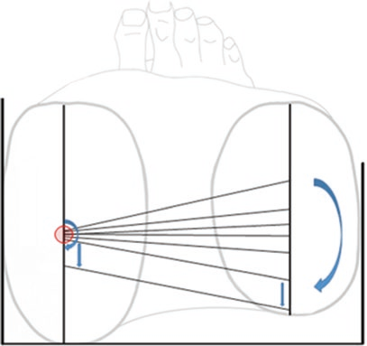
From 0° to 120°, this medial-pivot teaching model keeps the medial femoral condyle nearly stationary on the tibia. The lateral condyle translates posteriorly about 20 mm, coupled with about 20° of tibial internal rotation around a medial axis.
Iwaki, Pinskerova and Freeman mapped this pattern in unloaded cadaver MRI. Living-knee MRI studies by Hill and Johal found broadly similar asymmetric motion under unloaded and loaded conditions; loading can bring rotation forward in the flexion arc. Fluoroscopy studies, including Komistek, also show that individual knees and activities vary.
ANATOMIC RESURFACING HOW THE NATIVE KNEE FLEXES
Native knee: medial stability, lateral rollback.
Right knee · Full extension
Preparing the 3D knee…
Medial condyle Medial plateau · concaveLateral condyle Lateral plateau · flat / slightly convex Fibula marks the lateral side
Both sides move. Watch the lateral side travel farther back.
0° FLEXION
Medial stays close. Lateral travels back.
Follow the blue arrows: the medial center stays close to its starting point while the lateral center travels backward.
Medial · MCLLateral · LCL
Modest medial travel
← Posterior
Greater lateral travel
← Posterior
Preparing the close-up views…
Blue arrow · center travelPink trail · contact estimate from 35°
0° flexion
Illustrative pattern · medial movement begins gradually around 35° here; timing varies between knees and activities.
Both blue travel tracks use the same scale. The open pink ring marks the contact estimate at 35°; the solid dot marks its current position.
What the animation represents
This prescribed teaching example keeps the medial posterior reference center nearly fixed in the anteroposterior direction through 35°, then gradually introduces 3 model units of posterior movement by 120°. Coupled rotation gives the lateral center substantially greater travel. These values and the 35° onset were chosen for the illustration; they are not universal thresholds or measurements from a published cohort.
Published findings vary with loading, activity, rotation and measurement method. Freeman and Pinskerova emphasize medial stability through the main flexion arc; Johal reported minimal medial posterior translation until approximately 120°, while Hill observed some anterior medial movement during loaded squatting. This animation demonstrates relative stability and possible modest motion, not a single path followed by every native knee.
Blue dots track the actual transformed posterior condylar reference centers. Dashed lines stay fixed at their full-extension AP positions. Pink markers and their trails are geometric surface-proximity estimates sampled from the seated model, not measured cartilage contact or pressure. The open pink ring stays at the 35° estimate, separating early contact transfer from subsequent travel; the trail is identical when scrubbing or playing backward. Blue arrows show center displacement from the fixed extension line. Both projections face the same direction at the same scale. The original anatomy and seating guard are retained; this is not a validated biomechanical simulation.
The circle marks the posterior flexion-facet center. The pink marker follows the nearest opposing surfaces in this model as it flexes. Watch the surface marker separately from the center.
Preparing the knee…
MEDIALLATERAL
0°
0° / 120°
Pink is a geometric proximity marker, not measured cartilage contact or pressure. The published early contact transfer is a teaching distinction; this specimen’s marker is computed from its surfaces.
One knee. More than one motion.
Loading, rotational position and the depth of the bend change the movement. These study diagrams separate those effects from the illustrative 3D knee.
Unloaded bending
Weight-bearing squat
Start together, then watch the lateral centres separate.
Pinskerova et al. (2004), Table I · The same five volunteers in both conditions. Dots show each flexion-facet centre’s travel relative to extension, with starting positions aligned for comparison. The outlines and connecting lines are schematic, not measured femoral orientation. Movement between measured positions is interpolated.
Read the evidence and its limits
Hill et al. (2000) examined 13 unloaded living knees and seven loaded knees. The loaded group showed about 4 mm of medial forward movement. In four knees tested with altered rotational positioning, tibial external rotation suppressed the usual accompanying internal rotation during squatting to 90°. This is a separate cohort from the five-volunteer comparison above; the datasets are not interchangeable.
Iwaki et al. (2000) studied six unloaded cadaver knees. Their pattern included early axial rotation, comparatively little additional rotation to approximately 45°, and greater rotation later. The 3D patient animation uses an illustrative phased trajectory based on this description, not digitised individual-knee data.
Contact location is not condylar translation. Pinskerova et al. measured contact as the closest approach of the subchondral plates on MRI. This is not a pressure map or the full cartilage–meniscus load-bearing area. These related studies and the later review do not establish one universal trajectory, ligament-force behaviour, or clinical outcomes after resurfacing.
Sources, measurements, and what this animation represents
The live values are prescribed animation targets, not measurements from this specimen. Medial AP is the flexion-facet-center translation, not the migrating contact point. The animation uses 1 mm medial and 20 mm lateral posterior translation with 19.9° coupled rotation at 120°. The sagittal overlays identify the flexion-facet centers; they do not represent contact patches. The bone positions include a geometric surface-clearance correction, not a force-based cartilage simulation.
The medial-pivot pattern is a teaching reference, not an invariant rule. Hill reported approximately 4 mm medial forward movement in loaded knees. Komistek studied five knees and reported individual variation, including a lateral-pivot subject. These studies do not establish that every native knee has no medial rollback or that loading affects timing alone.
[S15] Hill et al. (2000) ↗Hill PF et al. · 2000 · Living-knee MRI studyScope & limitations — loaded and unloaded living-knee MRI; similar overall pattern with load-related differences.
[S17] Freeman & Pinskerova (2005) ↗Freeman MA et al. · 2005 · Anatomy and kinematics reviewScope & limitations — 0–120° medial stability, early contact transfer and lateral rollback; deeper flexion is outside this film.
Bone geometry: Open Knee(s), specimen oks009, mirrored to a right-knee teaching reference. Articular surfaces and ghosted menisci are illustrative. Geometry, animation license and adaptation details. This is not a patient-specific or validated joint-contact simulation.
Medially constrained polyethylene
Stable medially. Free to rotate.
Medial conformity helps control anterior-posterior motion. A less conforming lateral surface permits travel around it.
01 Geometry guides motion
Preparing the implant…
Medial containmentLateral travel
Medial containment.
Greater conformity resists AP translation. The medial side still has some motion.
Lateral freedom.
A less conforming surface allows the lateral condyle to travel as the knee rotates.
The femoral component and insert work together. Conformity alone does not guarantee a medial pivot.
90°
Illustrative implant mechanics, not measured kinematics. Original educational 3D geometry, not manufacturer CAD. The medial socket represents a matching construct, not every MC insert.
02 The other half of the bearing
The lateral surface matters.
Lateral freedom. Contact support. A flatter sagittal surface permits travel; a posterior upslope changes the available path and support.
Preparing the implant…
Flatter lateral surfacePosterior upslope
Two illustrative constructs, shown at the same flexion. Their movement is prescribed for teaching, not a measured comparison or a prediction of wear.
The study behind the comparison+
Delman et al. · 2021
Bilateral comparison · 25 patients · KA
The medial ball-in-socket/flat lateral construct maintained a medial pivot. A posterolateral upslope was proposed to explain different motion with the low-conforming CR construct.
Different implant systems, PCL management, and follow-up. No difference in median patient-reported outcomes.
Reduced conformity can concentrate contact stress. Medial lift-off may overload the less-conforming lateral side. Unfavorable contact near a bearing edge is a further concern.
Preparing the implant…
Medial lift-offLateral load concern
Exaggerated medial lift-off at a fixed bend. The amber marker identifies an area of concern; it is not a pressure map, wear measurement, or simulation result.
Contact stress, edge loading, and wear+
A smaller contact area may increase local stresses, but higher stress alone does not establish greater clinical wear. Edge loading also depends on contact location, component position, and compartment separation.
In 16 well-functioning GMK Sphere knees, medial separation was rare and mostly occurred in non-weight-bearing activities. The study discussed lateral overload as a concern; it did not demonstrate accelerated wear. The lateral bearing was sagittally flat and partially conforming coronally.
The bearing guides motion within the reconstructed knee. Its behavior depends on the joint line, component position, and soft tissues.
Medial congruent ≠ medial pivot+
Medial congruence describes surface conformity. A true medial ball-and-socket construct pairs the insert with matching femoral geometry. “Medial pivot” can describe a design concept or an observed motion pattern.
These terms overlap, but the geometries and resulting movements are not interchangeable.
PCL retention or resection is specific to the implant construct and surgical plan. These studies do not establish a universal PCL strategy or show that medial conformity replaces collateral ligament function.
A conventional femoral component placed in greater valgus and less external rotation can move the trochlear groove medially. The patella then rides more laterally relative to the groove, changing its engagement.
Compare native tracking, a level mechanical-alignment reconstruction, and a resurfacing example with a component-design mismatch. Resurfacing does not inherently cause poor tracking: a design suited to the intended alignment can address this mismatch.
The cited study compared component geometry on ten 3D models. It did not measure clinical patellar tracking or complication reduction.
Centered engagement with a conventional component in this example.
03 · AP
Valgus Implant Placement
Implants · 5° varus joint line
Loading anatomy…
LateralMedial
The groove angles medially. The patella rides lateral to it.
Trochlear groove & joint linePatellar center trackFixed AP · synchronized motion
Extension
The tibia bends away from the fixed AP camera as the patella descends. Its depth is retained and the tibial bearing moves with the bone. The patella is semi-transparent so the trochlear guide remains visible through it.
Illustrative AP projection using a textured tibial volume and prescribed patellar excursion—not a 3D biomechanical simulation or a predicted outcome. The tibial shape and ligament paths are approximate. The third example uses a conventional mechanical-alignment component in greater valgus and less external rotation. Its 5° varus joint line is an example, not the cause of maltracking by itself. Implant design, rotation and soft tissues also matter.
The sunrise perspective
See the rotation. See the tracking.
From this axial view, compare the patella’s position over the native trochlea and the trochlear implant. The native and mechanical-alignment examples share the same rotation and centered tracking.
The third example shows a slightly internally rotated femoral component with the patella displaced and tilted laterally. It illustrates a positioning mismatch to recognize—not the expected result of anatomic resurfacing.
The illustration is a teaching example, not a reproduction of this study’s result. Ko et al. found no significant difference in patellar tilt between rotation groups when using the gap technique with ligament balance.
Illustrative axial projection, not a radiograph or patient-specific simulation. The first two examples share the same rotational reference. The third deliberately combines internal rotation with lateral patellar subluxation and tilt to demonstrate a possible mismatch—not an inevitable outcome of resurfacing or a degree-based prediction. Tracking also depends on component design, tibial rotation and soft tissues.
Surgeon library & exchange
Publications, presentations, and cases
Explore the literature. Share a presentation. Walk through a case.
Broader reference material and papers whose filenames do not identify a specific subject. Topics are based on available filenames and collection labels, not a full-text review.
PDFs open at their original location with existing access permissions. Some require an authorized Microsoft account; inclusion here does not grant access.
This library includes research articles and supporting reading. Inclusion is not an endorsement of a study’s conclusions; filenames are not verified citations.
Polyethylene
1,876 references · 711 PDF links
Knee insert design: medial congruence, medial stabilization and constraint, with related bearing designs listed separately.
Imported from the supplied knee insert reference collection, compiled September 11, 2026. Citations and design tags are preserved from that collection. Its search covers PubMed/MEDLINE; categories reflect indexed terms and are not a full-text assessment of each paper.
PDF links open the original publisher or repository locations recorded in the supplied collection, which identifies these papers as open access. Availability is controlled by those sources. References without a downloaded PDF retain their publisher and database links. Inclusion does not establish clinical superiority.
Educational contributions are not peer-reviewed guidance or a substitute for clinical judgment. Contributor names and credentials are self-reported. External links retain their own access settings.